
Why This Article?
This article is a continuation of Are your industrial data science models field ready? – Part 1: How Low is Too Low for R2. If you have not read it, please go to link
In the last section, we talked about how to decide the success criteria for your models. Now, let us look at how
to build models that will match up to their lab promises when transitioning to the field.
It is important to test the generalizability of your models by using techniques like cross validation. This is
where we train our model on a portion of the data and use the remaining portion to check the model’s
performance on the unseen data. This is a well-known idea, and you can refer to any machine learning
book for details. However, there are some nuances to this approach that are not apparent. I will start
this section with a real-world example to help ground the discussion.
Real World Example
Our team was tasked to build a diagnostic model for industrial equipment to recognize faults before the
tool was deployed on a new job. I was part of a large and incredibly talented team of data scientists. The
fault data was limited, and we used robust techniques, including cross validation, to ensure the models
are generalizable. We obtained some exciting results and deployed the model on the field.
Unfortunately, it never worked in the real world. There was not a single instance where it could correctly
identify a faulty equipment and not a single instance where instances flagged by it corresponded to
faults. Like the lead character in the movie A Beautiful Mind, we saw patterns that did not exist. This
created a poor reputation for machine learning as a useful technology at the company. Luckily, most of
us moved on from this project without significant career damage. Years later, I mulled about what went
wrong and below is the explanation
A Small Contrived Example
Let us start with an experiment. Here is a dataset
(http://deepiq.com/docs/dataset1.csv) that pertains to
figuring out if a pipeline has a crack in any cross section of
interest. We used a non-destructive evaluation equipment
with four different sensors that take measurements from each
cross-section of interest along the pipe.

All the historic data was persisted to a PI Historian and the field
engineer used the PI Historian’s Asset Framework Expressions
to calculate the average value of a sensor from each cross
section of interest, and saved as “sensor i-tag one” in the
dataset.
We are charged with building a model to diagnose cracks based
on these sensor readings. So, we must build a model to classify
each area into a “no crack” (label one) and “crack” (label zero)
after dividing the data into train and test. I request you to read this section before attempting the
exercise because there is a gotcha element to it.
I used the following approach.
- Split the data into 80%-20% for train and validation datasets, making sure both positive and
negative sample ratios are preserved in both sets. - Build a decision tree using the train set and validate it on the validation set
I ended with a validation error of 0.55 and a train error of 0. The model is over trained and is performing
worse than a random number generator on the test set. Bad results. Luckily, the field engineer was a
believer in the promise of machine learning, and he was open to deriving additional statistical metrics
from the raw measurements recorded in PI. Using his domain knowledge, he used PI Expressions to
derive additional features based on the raw sensor measurements. Each sensor collected around 1,000
measurements from a cross-section of interest and literally there are quadrillion ways of calculating
features. So, we focused on an iterative model development. He extracted a set of possible features and
I ran my machine learning pipeline on the features to calculate performance metrics. Luckily after a few
iterations, we found a fantastic model with a training error of 0 and test error of only 0.15. The final set
of all features we iterated through is in the dataset, dataset2.csv and my best
results were obtained for the following features:
- Sensor 1 –Tag 2
- Sensor 2 –Tag 3
- Sensor 3 –Tag 1
- Sensor 4 –Tag 3
We found a great candidate that is viable for field deployment with some nice teamwork!
Here is the caveat. All sensor readings and labels in the dataset were generated using a random number
generator. In other words, there was no predictive value in any of the readings. At this point, if you want
to experiment with this data, please go ahead. I did not want to waste your time on random data
exploration. The model I found is predicting random numbers.
This is a contrived example and based on a small number of data points. It is easy to see where I messed
up. We have only 20 points in the test data set and a random label generator has more than 0.5% chance
of having higher than 80% accuracy and more than a 2% chance of having higher than 75% accuracy on
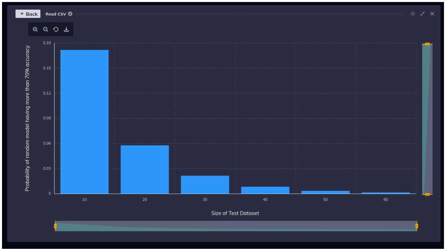
test data. To check if this issue occurs in slightly larger data sets, let us consider a binary classification
problem where both classes are equally likely, and features have zero discrimination capability. Now, let
us calculate the probability that a model which assigns label randomly has more than 70% accuracy on
the test data. The probability falls quickly with an increase in the size of the test data set and is only
0.13% for datasets of size 60. That is good news. You can still build robust models on small datasets.
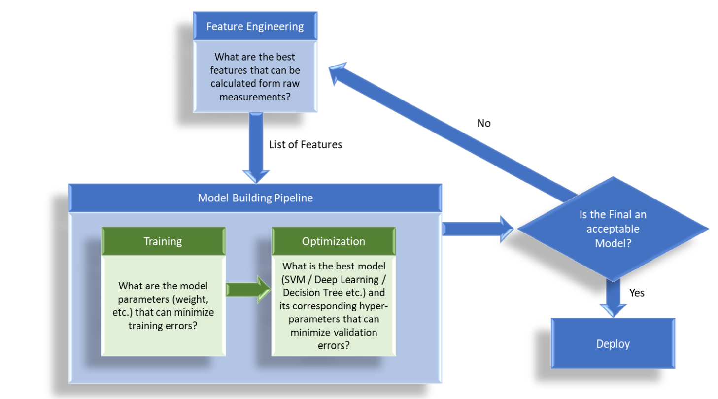
Here is the catch though. Consider your stand machine learning pipeline (Figure 3). The steps are:
- Data Engineering: In standard industrial analytic use cases, we will need to do significant data
preprocessing to build analytic ready datasets. For example, you might have to interpolate your
time series data from different sources to map them to a single frequency using statistical
techniques. We might use parameterized physics-based equations to derive additional signals
from raw measurements based on domain knowledge. Other standard steps include normalizing
the data, doing dimensionality reduction, and performing data cleansing operations to improve
feature quality (such as data imputation to handle missing data, smoothing to handle noise, and
outlier filtering to handle faulty readings). Some of these steps might be bundled into our
hyperparameter tuning exercise and checked against a final test set to obtain an unbiased
estimate of the generalization error. However, more often than not, some of the data
preprocessing steps are handled outside the model building loop and therefore not locked away
from a final check against a test dataset. - Training Algorithm: Using cost minimization functions like back propagation (for neural
networks) or least squares minimization (for regression), this step finds the model with the
lowest error on the training data set - Model Optimization: The model optimization component deals with finding the right model
(decision tree vs. deep learning model, etc.) and the right hyper-parameters (no of layers in your
neural network or number of trees in your random forest, etc.), to maximize the performance
on the test data set. In this step, we enumerate multiple models to find the model that has the
lowest validation error on the validation dataset (or using cross-validation). Techniques like grid
search that exhaustively enumerate different combinations of parameters or smart search
algorithms that rely on some greedy heuristics to prune the search are used to find the model
with the best performance. AutoML techniques on standard platforms provide an abstraction
layer for this step so you do not need to bookkeep the cumbersome search process.
Now, count the number of model trials you are attempting due to the combined iterations of data
engineering, model type search and hyper parameter tuning exercise. If these trials add up to a million,
then even with a 60-size test dataset where we previously computed the probability of a completely
random model producing more than 70% accuracy as 0.13%, the expected number of models with at
least 70% accuracy is more than one. If you include the fact that automated techniques like AutoML use
a smart search algorithm that use a greedy hill climbing exercise to minimize validation error, the
problem becomes worse.
You might argue that you always leave a test dataset untouched by the above optimization cycles where
you do a final check of your model robustness. While you are likely keeping the test run outside the hyper
parameter optimization step, are you adhering to the discipline of keeping the test run outside the data
engineering loop too? Many practitioners do not, particularly in industrial use cases, where there is
significant domain knowledge and cleansing operations that are involved in building analytic ready
datasets. That is, if you revisit your data engineering cycle when your test score is low, you will still run
the risk of contaminating test performance scores because of excessive data engineering.
Why is this more important for industrial data problems?
Businesses typically consider their problems as a given and data science projects as a tool that either succeeds or fails in solving this prescribed, constant problem. However, they leave value on the table by doing this. Optimal use of your analytic models might require you to adapt your business strategy and, in some cases, completely change your business model.
A Small Contrived Example
This phenomenon occurs more often than you might think in industrial data science because of the following reasons:
- Often in industrial data science problems, you might have large datasets but only a small set of
labelled samples to train your models on. For example, your compressor might be generating
hundreds of measurements every second but may have failed only once in the last two years. In
the above example, the number of cross sections of interest that have data to train on is only
100. - Within this small set of labelled samples, positive cases like faults are significantly smaller than
the normal cases. So, you end up with a biased dataset where most labels are same and your
models learn that by predicting a constant value of the most frequent label, it will end up with
high accuracy. For example, if 95% of our cross sections of interest do not have cracks, picking
“no crack” as the predicted label always will have an error rate of only 5%. Since the baseline
accuracy itself is high, to test the model generalizability, we are trying to optimize a needle in a
haystack. - In addition to the lack of labelled examples, in industrial use cases, there is significant data
engineering that is a precursor to the machine learning workflow. In machine learning problems
such as computer vision, deep learning models directly operate on the raw pixel data and
intrinsically compute the features required by the model. Contrast this with a standard industrial
data science problem. Using parameterized physics or domain equations, computing statistics of
raw features, decomposing signal to frequency components, smoothing, interpolating data to
change scale etc are routine procedures that are usually handled outside the model optimization
loop. These provide a high degree of freedom to data scientists even before machine learning
processing with AutoML tools. In many industrial analytic problems, problem formation and data
engineering remain the secret sauce of success.
The advent of enormous computation power that allows you to iterate through millions of data
engineering cycles in an iterative process as an input to your AutoML or other model search processes,
creates the artefacts that we saw earlier. When your model fails, a natural response is to engineer better
data. This is a useful exercise. However, as you try out hundreds of pre-processing steps, hundreds of
models and hundreds of hyper parameters with automated tools, the danger of the phenomenon that
you observed in the last problem becomes real.
If your labelled samples are small and generating your dataset involves significant data engineering that
is outside your model test performance runs, you might inadvertently overhype the quality of your
resultant model. If you are doing considerable data engineering as a pre-processing step to your machine
learning pipelines, the responsibility of making sure that the number of combinations and permutations
you throw at your machine learning pipeline does not undermine the validity of your results stays with
you. You will need an application that treats the end to end pipeline from connecting to your raw
sources to producing the final insights as one holistic process that is handled within your model
optimization cycle.
How DataStudio Helps
In a typical industrial data science workflow, you will have to put in significant work to build machine
learning ready datasets. Your analytic workflows will have a large pipeline where model building is usually
the last and easiest step. Typically, your AutoML/data science tools stay out of the first phase of data
engineering, making controlled optimization of the entire analytic process difficult.
DataStudio is the first self-service analytics application that gives you the ability to connect directly to
your IOT and geospatial sources and perform highly scalable feature computation, feature ranking,
model selection and hyper parameter search using a simple self service application. Using our hyper
parameter optimization capability, you can easily iterate through multiple data engineering and model
parameters in a single optimization cycle, while keeping a fine-grained control on the risks of over
optimizing the model that can damage its generalizability.
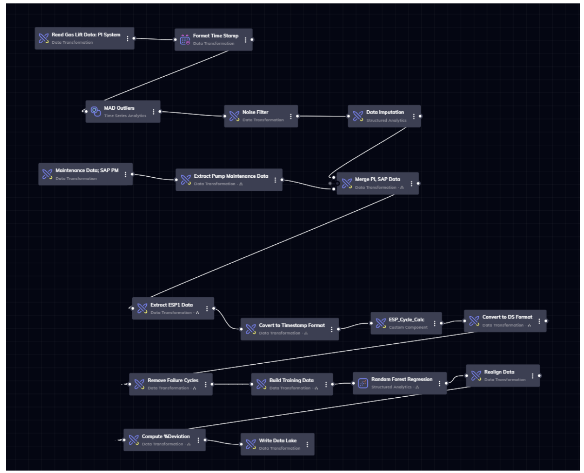
Figure 4 shows a workflow that we built to explore machine learning approaches to detect anomalous
behavior in a field pump operation to prevent catastrophic failures. The actual details of our workflow
are available in this video ml.mp4 but we provide a overview to showcase how
feature computation and model building operate together in an industrial workflow. In this workflow,
first we select a set of tags that we consider relevant to this problem and pull the data from PI historian.
Then, we remove outliers to account for any malfunctioning sensors. We use a noise filter to remove
high frequency noise. Then, we use an imputation algorithm to fill out missing data with a statistical
algorithm. All these are parameterizable components that you can experiment with to give you the best
result.
Finally, in the bottom part of the workflow, the actual machine learning model building process beings.
We merge the PI data with maintenance data from SAP to get labelled examples and use a grid search
algorithm to find the best possible Random Forest model
This single workflow goes all the way from connecting to your IOT sources, to generating finished models
and can be optimized for best generalization metrics. Now that we saw how to build good models, in the
final part of our article, we will talk about how to combine your high performing models to create the
“best of the best” model.
For further information, please contact us at info@deepiq.com
Download the whitepaper here