Data science for industrial digital transformation Hype or Hallelujah? – Part 3

Why This Article?

This article is a continuation of Are your industrial data science models field ready? – Part 2: How Low is Too Low for R². If you have not read it, please go to resources page

In the first two sections, we talked about how to establish success criteria for your models and how to
avoid building models that will have poor performance in the field. Now, that you can build some high-quality models, how do we combine your models to optimize their performance? This article provides a
deep dive into this topic.

While building your models, you might end up with multiple models that you like. Your legacy reasoning
tools, or human experts may be providing alternate predictions. An obvious approach to combine the
model results is to average them out, with an idea that the errors will cancel out. The intuition is strong
and driven by the central limit theorem that states that the mean of a sample of data will be closer to
the mean of the overall population as the sample size increases, notwithstanding the actual distribution
of the data. So, when we have multiple unbiased models that are independent, their average prediction
will average out to be the correct value.

While this is a powerful intuition, it does not hold sufficiently for machine learning model fusion. The
main reason is that our models are typically not independent or identically distributed, which are
requirements of the common form of the central limit theorem.

For a first example, let us assume that we have two models that generate independent predictions,
conditioned on the true value of the predicted variable. Both models are unbiased, and the errors have
normal distributions with different variances as show in table 1 ( the model generated predicted
value is the true value of output variable). Now, let us average out the two predictions to get a
fused prediction for the variable of interest. Since the sum of independent, normal distributions is also a
normal distribution, the fused model will have the distribution shown in table 1.

Is the quality of the fused model better than the original model? That is, does our fused model have a
lower error variance than the individual models? Consider two scenarios as shown in table 2. In the first
scenario, both models are identical. In the second scenario, model 2 is better than model 1. The fused
model is better than both models in the first scenario but worse than model 2 in the second scenario. In
the second scenario, fusion negatively impacted our final performance.

Is there a better way to fuse models? Is there an advantage we can derive by combining a good model
with an inferior model? Turns out there is. Let us start with a simple contrived example where we
combine multiple models with varying quality to create a model that is better than all of them.

A Small Contrived Example

An industrial floor is being monitored by three
sensors to prevent safety incidents, so that we can
trigger an alarm if a person is entering the area of
operation when heavy equipment is being used.
There are three different sensors that are being
used to monitor if a person is entering an active
area of operation:

• Audio
• Infrared
• Video

A Small Contrived Example

Let us start with an experiment. Here is a dataset
(http://deepiq.com/docs/dataset1.csv) that pertains to
figuring out if a pipeline has a crack in any cross section of
interest. We used a non-destructive evaluation equipment
with four different sensors that take measurements from each
cross-section of interest along the pipe.

Each of them has an embedded model that process the raw sensor feed and generates an output of 1 if
they detect a person entering an area of interest, or 0 otherwise. The video sensor model is fantastic at
detecting persons with probability of missed detection (P_md )= 0.1, but has a problem with false positives,
with probability of false alarm, P_>fa = 0.5. The audio sensor is bad at detecting a person (P_md = 0.6) but is fantastic at filtering out false positives (Pfa = 0.2). The infrared sensor is mediocre at both tasks, with both
probability of missed detection (P_d) and probability of false alarm (P_>fa) equal to 0.4. Conditioned on the
event of interest (person entering the area of interest), all three sensors are independent. Both the
events, person in an area of interest and not in area of interest at any instant, have equal priors of 0.5. If
your final objective is to minimize the total error of prediction, what is the best way to fuse the readings
to produce the prediction?

If you use the infrared sensor alone to decide on the presence of a person, it is easy to see that your error
probability is 40% on average. If you use the video (sound) sensor alone, your error probability is 45%
(50%). Let us use Bayes theorem to calculate the posterior probability of the presence of a person for
each possible set of observations as a first step

The probability that a person is entering the area of interest given that we record certain sensor readings
x_video, x_audio, x_infra can be calculated as:

The results of the application of Bayes theorem to each possible set of sensor readings are shown in table

Let us do a simple fusion rule where we average out all three sensors and calculate what your error
probability will be. Table 3 shows the results of our simple fusion algorithm, the model average
algorithm, that averages out all sensor readings and rounds the output to the nearest integer. The
average decision rule is the same as the maximum voting rule for binary classifiers. Let us calculate the
probability of error for this algorithm by comparing the probability of presence of a person and the
decision we will make on presence of a person using the model average fusion output. Your chance of
making a mistake in this case will come out to be 30% and this is significantly better than using any one
sensor alone. This turns out to be our lucky case when averaging the models was better than using any
one of the models. But is this the best we can do?

For the optimal fusion rule, let us pick the class with the highest probability of occurrence given a set of
sensor readings since that clearly minimizes the chance of us making an incorrect decision. As you can
see, the maximum voting rule/model average rule and the optimal fusion rule produce the same output except for the scenario when the video sensor says there is no person and the other two sensors say
there is. In this case, the optimal fusion rule is predicting that there is no person, but the model average
rule is predicting that there is a person. If you look at class probabilities, you can see that the probability
of a person in this case is only 0.38. So, the model average rule would have been wrong 62% of the time
while the optimal fusion rule would have been wrong only 38% of the time.

Your overall chance of making an error using the optimal fusion rule is only 26%, which is better than the
model average rule at 30%. Clearly, the model average rule is leaving money on the table. The best fusion
algorithm you can use turns out to be a weighted sum of all the models and not a simple average

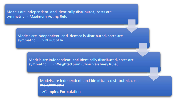
It turns out for the binary decision fusion; the math is easy to lay out. Depending on multiple criteria
including whether costs of errors is symmetric (the cost of false positive is the same as the cost of missed
detector), whether the models are identically distributed or whether the models are independent, there
is a hierarchy of fusion rules that will minimize the expected cost of error

• In the simplest case, all models are identically distributed and independent. In this case the
  maximum voting rule is the optimal fusion rule.
• The second case is that all models are independent and identically distributed but the cost of
  making certain errors is different for different types of errors. In this case, the best fusion rule
  turns out to be n of m models rule.
• The third case is all decision makers are independent but not identically distributed. In this case,
  the best fusion rule turns out to be weighted sum rule also known as Chair Varshney rule.
• Finally, we have the worst case and the most usual case for machine learning model fusion. In
  most real-world machine learning scenarios, we are struck with the complex case where:
  • Models are not independent
  • Models are not identical
  • The final output is not binary but n-ary or real valued
  • The individual models are not similar in their outputs (some produce class labels and the others real numbers)

This is where machine learning comes to our rescue. Machine learning approaches can be used in almost
any fusion use case to great effect. The idea is simple – pose the model fusion as a learning problem,
where the feature vector is the vector of outputs of each model and the fusion output is the true value
of the variable you are trying to predict

In industrial analytics, while a single model might dominate others in terms of standard machine learning
metrics like R²
or accuracy, other models might have better performance on business specific KPIs. For
example, your legacy physics model might be better for predicting steady state performance. A vendor
provided model might be better at predicting certain failure types. Using fusion, you can train a model
to combine the best characteristics of these individual models into a single globally dominating model.

To this end, you will need an application that allows you to build, manage and compare multiple
models based on multiple business driven KPIs and combine the best of them for optimal outputs.

Are there any caveats here? Yes. All the limitations of machine learning apply. An obvious issue with
combining models is overtraining. You must use rigorous cross validation technique to ensure models
are generalizable.

A Real-World Example

Businesses typically consider their problems as a given and data science projects as a tool that either succeeds or fails in solving this prescribed, constant problem. However, they leave value on the table by doing this. Optimal use of your analytic models might require you to adapt your business strategy and, in some cases, completely change your business model.

A Small Contrived Example

These are results that we published in my 2012 paper (Tumu et al)

The idea is to detect the depth of each pixel from a single image without using additional images of the
scene. At that time, there were two seminal papers that dealt with this problem.

• One of the models was called make3D, and it predicts the exact depth of each image pixel.
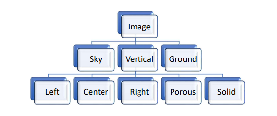
• Another paper HEH classifies images into a set of geometric classes related to 3D structure as
  shown in Figure 2.

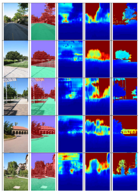
Figure 3 is the result of fusing the results of both the models using a random forest regression model. A
comparative visualization of the depth was estimated generated by Make3D and the fusion approach.
From the left, the first column shows the original image. The second column shows the labels generated
by HEH. The third column shows the depth map produced by Make3D. The fourth columns show the
depth map generated by our fusion of Make3D and HEH. The final column shows the ground truth.

As you can see, the fusion improved the quality of predictions. Figure 4 shows the decrease in error
obtained by the fusion as compared to Make3D per HEH class label. Interesting improvements for all
classes of data considering we were trying to improve the baseline of the then state of the art models.

How can DataStudio Help?

In many use cases, you will end up with multiple models with competing strengths. For example, you
might have an expert developed rule-based model that is producing excellent results in predicting your
compressor health within surge and stonewall limits. Your own custom machine learning model might
be better outside these operational limits. With DataStudio, you can build multiple models with varying
strengths by using combinations of feature engineering, data sampling and model selection techniques.
You will bring all your models into a single application and rank them not only using standard machine
learning metrics like accuracy or overall error, but also using additional business specific KPIs like impact
on HSE, performance by region, asset type etc. Since all the models are persisted in a simple to use
DevOps application, you can retrieve them and regenerate results as input to your fusion model. Figure
5 shows the model management page for DataStudio where the models generated by different
experiments are listed. You can compare all your models in a single view, select models that are non-dominated by others and build a model of models to get the best of all worlds.

Conclusion

Some of the details we presented in this article series are rather intricate and we barely touched the surface on
the possible approaches to address them. The key takeaway to highlight is that your industrial data science
needs are unique. To deliver value at scale with AI, you will need a specialized software that addresses these challenges. I have seen many industrial companies use general purpose AI software for their digital programs.
I can confidently state that in many cases, their models are not field ready, or they are leaving money on the
table. DeepIQ’s software is built to make your industrial data science simple and powerful. Please contact us at
info@deepiq.com if you are interested in a deep dive.